Welcome to our Q-Learning tutorial! This guide provides an in-depth look at Q-Learning, a model-free reinforcement learning technique that empowers intelligent agents to learn optimal strategies in complex, dynamic environments. Whether you're new to reinforcement learning or looking to refine your knowledge, this tutorial has something for you.

In This Tutorial, We Cover:

• Introduction to Q-Learning: Understand what Q-Learning is and how it fits into the world of reinforcement learning.
• True Learning and Decision Making: Discover how Q-Learning agents make decisions based on rewards and future outcomes.
• Supervised vs. Unsupervised Learning: Explore the key differences between supervised and unsupervised learning, and why Q-Learning is ideal for environments requiring adaptability and long-term optimization.
• Q-Table Representation: Learn how Q-Tables are used to store and update an agent’s knowledge about actions and states, helping it make informed decisions over time.
• Visualization and Dataset Overview: Get an overview of the dataset used and how to visualize it for better understanding and learning.
• Creating the Churn Prediction Environment: Walk through how to set up a custom environment, such as a churn prediction model, to train your Q-Learning agent.
• Initializing Learning Parameters: Learn how to define and initialize key parameters like the learning rate and discount factor that guide the agent’s learning process.
• Training the Learning Agent: Dive into the practical steps of training your Q-Learning agent, observing how it improves decision-making over time.

Introduction

Q-learning is a key concept in Reinforcement Learning (RL), a fascinating branch of Machine Learning (ML). While traditional ML focuses on teaching computers to learn patterns from data, RL takes a different approach—it trains agents to make decisions by interacting with an environment to achieve a specific goal.

What Makes Q-Learning Unique?

Q-learning stands out as one of the first model-free reinforcement learning algorithms. Being model-free means the algorithm doesn’t need prior knowledge about the environment’s rules or dynamics—it learns solely through trial and error. This ability to adapt without predefined models makes Q-learning versatile and widely applicable.

Where does Q-learning fit in?

Imagine teaching a robot to play a game. At first, the robot knows nothing about the rules or strategies. Through trial and error, it learns by receiving feedback:

• Rewards for good moves.
• Penalties for bad moves.

The robot’s goal is to develop a strategy—known as a policy—that maximizes its total rewards over time. Q-learning is the technique that helps the robot estimate the value of each possible action in a given situation.

The "Q" in Q-Learning

The "Q" in Q-learning stands for Quality, referring to how beneficial a particular action is in a given state. To make this determination, the agent maintains a Q-table, essentially a cheat sheet where:

• Rows represent all possible states (e.g., the current situation in the game).
• Columns represent all possible actions (e.g., moves the robot can make).
• Cells contain Q-values, which indicate the long-term benefit of taking a specific action in a particular state.

How the Q-Table is Updated

The Q-values are refined over time using a formula that combines:

1. Current reward: Immediate feedback for an action.
2. Future rewards: The potential benefits of future actions.

Over time, the agent refines the Q-values to learn the best possible actions in every situation, achieving the optimal policy.

Predecessors of Q-learning

To better understand Q-learning, let’s compare it with other machine learning approaches:

‍Supervised Learning

• How it works: Models learn from labeled data to predict outcomes (e.g., fraud detection).
• Limitations: Effective for classification and regression but unsuitable for scenarios with unknown or evolving outcomes.

Unsupervised Learning

• How it works: Models uncover hidden patterns in unlabeled data (e.g., customer segmentation).
• Limitations: Great for exploratory analysis but incapable of handling sequential decision-making.

Reinforcement Learning

• How it works: Agents learn by interacting with the environment and maximizing cumulative rewards (e.g., robots navigating warehouses).
• Advantages: Designed for sequential, goal-oriented tasks, making it the ideal foundation for Q-learning.

How Does Q-learning Work ?

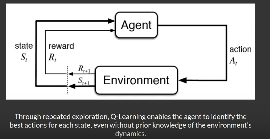
Q-learning involves a systematic process for learning the optimal policy through interaction with the environment.

1. Initialize Q-Table: Start with a table where every state-action pair has an initial value, often zero. 
2. Agent Takes Action: The agent selects an action using an exploration-exploitation trade-off:

• Exploration: Try random actions to discover new strategies.
• Exploitation: Use the best-known actions based on the current Q-table.

3. Receive Reward: After each action, the environment provides feedback—positive or negative—based on the action's outcome. 
4. Update Q-Table: Update the Q-value for the action using the Bellman Equation :

•  Q(s,a) ← Q(s,a) + α[r + γ max Q(s',a') - Q(s,a)]

Where:

• Q(s,a): Current Q-value for the state-action pair.
• α: Learning rate, which controls how much new information overrides old.
• r: Reward for the current action.
• γ: Discount factor, determining the importance of future rewards.
• max⁡Q(s′,a′)\max Q(s', a')maxQ(s′,a′): Maximum Q-value for the next state-action pair.

5. Blend current knowledge with new rewards and expected future rewards.
6. Repeat Until Convergence: The agent continues to interact with the environment, updating Q-values until they stabilize, indicating the agent has learned the best policy.

Code Implementation and Case study

We use the telecommunications dataset, specifically the Customer churn prediction using Telecommunications data , provided by IBM sample data sets.

This dataset contains information about customers of a telecommunications company, including demographic details, account information, and service usage patterns. The primary goal is to predict whether a customer is likely to churn (leave the service) or stay. By analyzing this data, companies can better understand customer behavior and take proactive steps to reduce churn.

Downloading and Understanding the Dataset

Let's start with downloading and understanding the dataset.

!git clone https://github.com/treselle-systems/customer_churn_analysis.git

We first install all the dependencies:

# Import Dependencies
import pandas as pd
import numpy as np
import matplotlib.pyplot as plt
import seaborn as sns
from sklearn.model_selection import train_test_split
from sklearn.preprocessing import StandardScaler, LabelEncoder, MinMaxScaler
from sklearn.metrics import classification_report, confusion_matrix, roc_auc_score
from tqdm import tqdm
import warnings
pd.set_option('display.max_rows', 500)
pd.set_option('display.max_columns', 500)
pd.set_option('display.width', 1000)
warnings.filterwarnings('ignore')

Next, we have a look at the data:

data = pd.read_csv('/content/customer_churn_analysis/WA_Fn-UseC_-Telco-Customer-Churn.csv')
data.shape

The dataset contains various features, including gender (male or female) and several categorical values such as online backup, data protection, and contract types (month-to-month or year-to-year). These categorical values will need to be converted or encoded into numerical values for analysis. Additionally, the dataset includes numerical features like tenure, monthly charges, and total charges. The target variable for prediction is whether a customer has churned or not.

Let’s do some quick EDA on the data set. We have all this information on the data set:

import matplotlib.pyplot as plt
import seaborn as sns


# Check data types and missing values
data_info = data.info()

# Get basic statistics for numerical columns
data_desc = data.describe()

# Check the distribution of target 'Churn'
churn_distribution = data['Churn'].value_counts()

Visualizing numerical features:

plt.figure(figsize=(10, 6))
sns.histplot(data['MonthlyCharges'], kde=True, color='blue')
plt.title('Distribution of Monthly Charges')
plt.xlabel('Monthly Charges')
plt.ylabel('Frequency')
plt.show()

‍

Visualizing categorical features:

plt.figure(figsize=(10, 6))
sns.countplot(x='Churn', data=data, palette='Set2')
plt.title('Churn Distribution')
plt.xlabel('Churn')
plt.ylabel('Count')
plt.show()

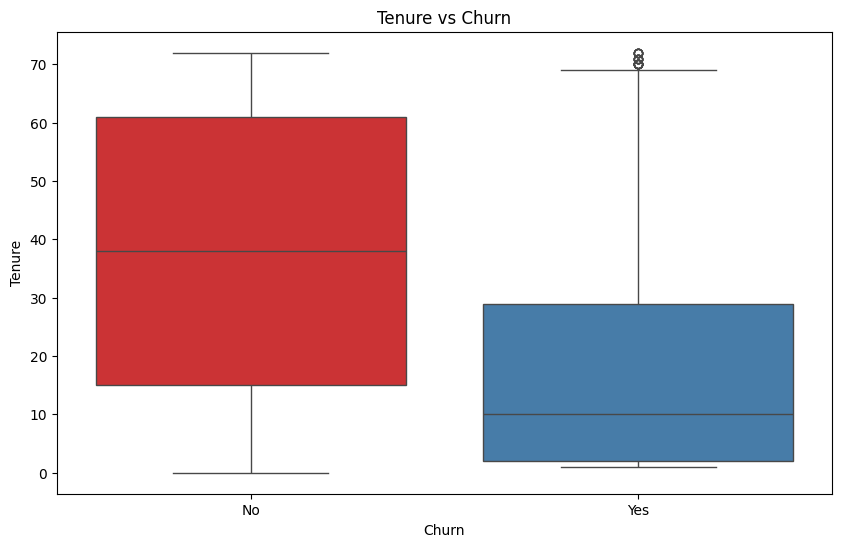
Visualizing the relationship between tenure and churn:

plt.figure(figsize=(10, 6))
sns.boxplot(x='Churn', y='tenure', data=data, palette='Set1')
plt.title('Tenure vs Churn')
plt.xlabel('Churn')
plt.ylabel('Tenure')
plt.show()

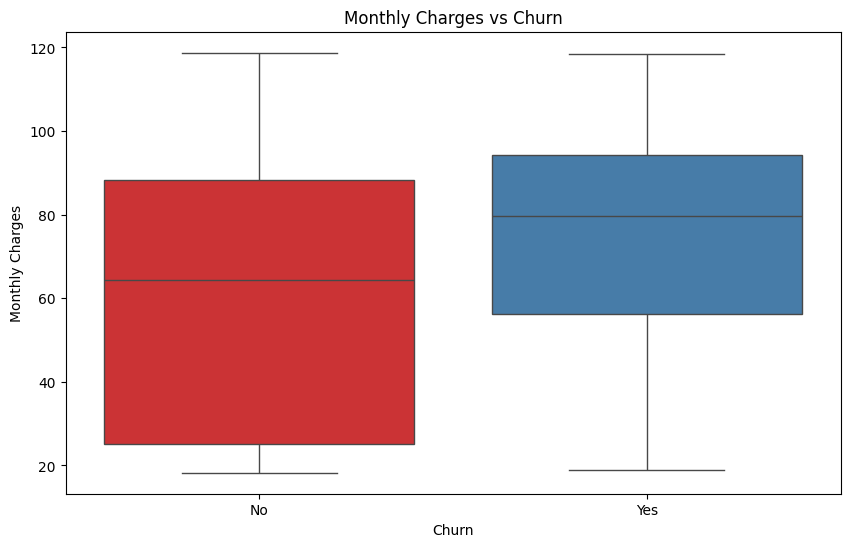
Visualizing the relationship between Monthly Charges and churn

plt.figure(figsize=(10, 6))
sns.boxplot(x='Churn', y='MonthlyCharges', data=data, palette='Set1')
plt.title('Monthly Charges vs Churn')
plt.xlabel('Churn')
plt.ylabel('Monthly Charges')
plt.show()

data_info, data_desc, churn_distribution

‍

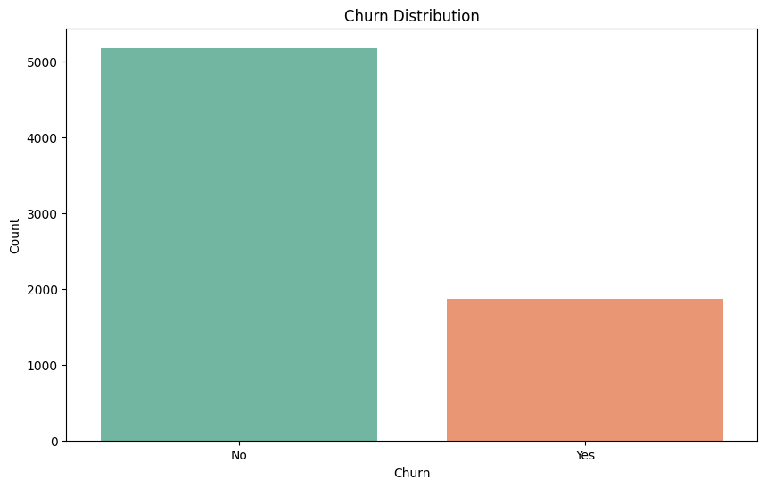
We can also see the distribution, which is fairly complex:

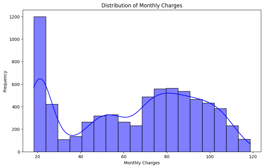
Next, we observe the churn distribution in the dataset. Approximately one-third of the customers have left the service, while the number of customers who did not churn is roughly three times higher.

We have the tenure versus churn distribution:

And We have monthly charges versus churn distribution.

Next, we move on to data preprocessing.

Data Preprocessing

We start by converting the categorical values into numerical values using a label encoder. The label encoder assigns unique integer values to each category, effectively transforming them into numerical representations.

def preprocess_data(data):
    # Convert categorical variables
    le = LabelEncoder()
    categorical_columns = data.select_dtypes(include=['object']).columns
    for column in categorical_columns:
        data[column] = le.fit_transform(data[column])

We scale the numerical features to a range of 0 to 1, which is more suitable for the Q-learning agent. The churn value, however, is excluded from this scaling process.

# Scale numerical features to [0,1]
    scaler = MinMaxScaler()
    numerical_columns = data.columns[:-1]  # All except Churn
    data[numerical_columns] = scaler.fit_transform(data[numerical_columns])

    return data

We load and process the data:

def load_and_preprocess_data():
    columns = ['customerID', 'gender', 'SeniorCitizen', 'Partner', 'Dependents',
               'tenure', 'PhoneService', 'MultipleLines', 'InternetService',
               'OnlineSecurity', 'OnlineBackup', 'DeviceProtection', 'TechSupport',
               'StreamingTV', 'StreamingMovies', 'Contract', 'PaperlessBilling',
               'PaymentMethod', 'MonthlyCharges', 'TotalCharges', 'Churn']

    data = pd.read_csv('/content/customer_churn_analysis/WA_Fn-UseC_-Telco-Customer-Churn.csv')
    data.columns = columns

    data['TotalCharges'] = pd.to_numeric(data['TotalCharges'], errors='coerce')
    data = data.dropna()

    return data.drop('customerID', axis=1)

After processing the data, all features are now numerical, and the customer identification column has been dropped. The dataset is fully scaled and encoded, and the churn data is ready for analysis.

For splitting the data into training and testing sets, we use a stratification technique. Stratification ensures that the proportion of the true label distribution (e.g., churned to not churned) is preserved in both the training and testing datasets. For instance, if the churned-to-not-churned ratio is 1:3, this ratio will remain consistent in both splits. This approach is particularly useful for imbalanced datasets, though more advanced techniques can also be applied.

The Softmax function:

def softmax(x):
    """Compute softmax values for array x."""
    e_x = np.exp(x - np.max(x))
    return e_x / e_x.sum()

Defining Q-learning agent class

Defining the Q-learning agent class begins with setting up a churn environment, which serves as the environment the agent will interact with.

class ChurnEnvironment:
    """Environment for the churn prediction Q-learning problem."""

def __init__(self, data):
        self.data = data
        self.state_dim = len(data.columns) - 1

In the constructor, we initialize the data values and the state dimensions. The state dimensions represent the features that the agent will observe. Specifically, we use the dataset's columns, excluding the policy data (indicated by data columns -1).

Next, we calculate the class weights. It is important to emphasize that misclassifying churners should be penalized more heavily than misclassifying non-churners. To address this, the weights are assigned dynamic values rather than static ones, ensuring appropriate punishment for errors based on the class imbalance.

# Calculate class weights
        class_counts = data['Churn'].value_counts()
        self.class_weights = {
            0: 1.0,
            1: class_counts[0] / class_counts[1]  # punishing misclassifying churners more than non-churners
        }

        self.reset()

We extract the state features, which convert the features of any given state into a vector representation. This allows the agent to process and learn from the state more effectively.

def get_state_features(self, state_idx):
        """Extract feature vector for given state index."""
        return self.data.iloc[state_idx].drop('Churn').values
        # state is a vector of numerical values that describe the customer

Next, we define the reset function, which initializes the environment at the beginning of each episode. It resets the done flag, indicating whether the training for the current episode is complete, and sets the current state to 0.

def reset(self):
        """Reset environment to initial state."""
        self.current_state = 0
        self.done = False
        return self.get_state_features(self.current_state)

We define the step function, which executes an action based on the agent's current state. The action the agent takes—whether to retain or not retain a customer—is determined by evaluating the features in the current environment.

def step(self, action):
        """Execute action and return next state, reward, and done flag."""
        # Executes an action (retention or no action) based on the current state
        current_row = self.data.iloc[self.current_state]
        actual_churn = current_row['Churn']

The reward system:

# Class-weighted reward structure
        if action == 1:  # Retention action
            if actual_churn == 1:
                reward = 5 * self.class_weights[1]  # Weighted reward for correct churner
            else:
                reward = -2  # Penalty for false positive
        else:  # No action
            if actual_churn == 0:
                reward = 2  # Reward for correct non-churner
            else:
                reward = -5 * self.class_weights[1]  
# Weighted penalty for missing churner

Let’s break this down in more detail:

• If the agent decides to retain the customer and the actual outcome is also retention (strength is 1), we assign a positive reward of 5, weighted by the class. This reflects a correct prediction of no churn.
• If the agent decides to retain the customer, but the customer actually churns (strength is 0), a negative reward of -2 is given to penalize the incorrect decision.
• If the agent decides not to retain the customer (no action), and the actual outcome is no churn (strength is 0), a positive reward of 2 is given. However, if the customer actually churns (strength is 1), a negative reward of -5 (weighted penalty) is applied for missing the churn.

After this, we calculate the next state based on the state dimensions. The done flag is used to indicate whether the episode has ended or not.

self.current_state += 1
        # next_state: The next customer’s features.
        # done: A flag indicating if the episode has ended (i.e., all customers are processed).

        if self.current_state >= len(self.data):
            self.done = True
            next_state = np.zeros(self.state_dim)
        else:
            next_state = self.get_state_features(self.current_state)

        return next_state, reward, self.done

Now, we get on to the Q-Learning agent.

The __init__ function has multiple parameters:

• state_dim: Represents the dimensionality of the state space, i.e., the number of features per customer.
• action_size: The number of possible actions the agent can take (in this case, 2 actions: retain or no action).
• learning_rate: Determines how much the agent updates its Q-values after each action. A typical default is 0.05.
• discount_factor: The agent’s consideration of future rewards, indicating how much weight it gives to long-term rewards. A common value is 0.99.
• epsilon: Represents the exploration factor in the epsilon-greedy strategy. It controls the degree of randomness in action selection to ensure that the agent tries different actions. The default value is 1.0.

class QLearningAgent:
    """Q-Learning agent for churn prediction."""
    # Class is responsible for learning the optimal policy (actions) based on the rewards it receives.

    def __init__(self, state_dim, action_size, learning_rate=0.05, discount_factor=0.99, epsilon=1.0):
        self.state_dim = state_dim                # state_dim: Dimensionality of the state space (number of features per customer).
        self.action_size = action_size            # action_size: The number of possible actions (2 actions: retain or no action).
        self.learning_rate = learning_rate        # learning_rate: How much the agent updates its Q-values.
        self.discount_factor = discount_factor    # discount_factor: The agent’s consideration of future rewards.
        self.epsilon = epsilon                    # epsilon: Epsilon-greedy strategy for exploration introduces randomness into the algorithm, forcing us to try different actions.
        self.epsilon_min = 0.15                   # Initially, epsilon = 1.0 (exploration-heavy). Over time, epsilon decays towards a minimum value (epsilon_min), encouraging the agent to exploit what it has learned.
        self.epsilon_decay = 0.999

        self.n_bins = 20
        self.q_table = {}

Initially, the epsilon value is set to 1, meaning that the agent will focus heavily on exploration. At the start of the Q-learning training, the agent should explore various actions to gather sufficient information. As the agent learns and updates its Q-table over time, the epsilon value gradually decreases towards a minimum of 0.15, following a decay factor of 0.999. By the end of the training, the agent will rely more on exploitation, using the knowledge it has gained to make the best possible decisions.

Discretization of the state:

def _discretize_state(self, state):
        """Discretize continuous state space into bins."""
        # Converts the continuous state (customer features) into discrete bins to manage large state spaces, else DQL
        binned_state = tuple(np.floor(state * self.n_bins).astype(int))
        return binned_state

The Q-table serves as a map that stores the Q-values for each state-action pair, essentially indicating the expected reward for taking a particular action in a given state. However, as state spaces grow larger, this can lead to significant space complexity. To manage this, we convert continuous customer features into discrete bins, reducing the size of the state space. Alternatively, we can use Deep Q-Learning, which employs neural networks to directly map raw features to actions, bypassing the need for a Q-table.

Now, based on the current state, the agent will select an action using the epsilon-greedy policy, which balances exploration and exploitation.

def get_action(self, state):
        """Select action using epsilon-greedy policy."""
        binned_state = self._discretize_state(state)

‍

We update the Q-table. This is where the Bellman Equation comes in:

def update(self, state, action, reward, next_state):
        """Update Q-value for state-action pair."""
        binned_state = self._discretize_state(state)
        binned_next_state = self._discretize_state(next_state)
        # ensures the agent’s Q-values converge to optimal policies.
        if binned_state not in self.q_table:
            self.q_table[binned_state] = np.zeros(self.action_size)
        if binned_next_state not in self.q_table:
            self.q_table[binned_next_state] = np.zeros(self.action_size)

        current_q = self.q_table[binned_state][action]
        next_max_q = np.max(self.q_table[binned_next_state])

        #Bellman Equation ->
        new_q = current_q + self.learning_rate * (reward + self.discount_factor * next_max_q - current_q)
        self.q_table[binned_state][action] = new_q

        if self.epsilon > self.epsilon_min:
            self.epsilon *= self.epsilon_decay

We update the Q-table using the Bellman equation and also update the Epsilon values.

Now we train the Q-learning agent:

def train_q_learning(env, agent, episodes):
    """Train the Q-learning agent."""
    rewards_history = []
    accuracy_history = []

    for episode in tqdm(range(episodes)):
        state = env.reset()
        total_reward = 0
        predictions = []
        actual = []
        done = False

Now, the agent will select an action based on its current state. Once the action is chosen, it will be passed into the step function, where the environment will process it and return the next state the agent enters.

while not done:
            # The agent selects an action based on the current state , make decision on that state with new action , update the state in q table , update the reward as well
            action = agent.get_action(state)
            next_state, reward, done = env.step(action)
            agent.update(state, action, reward, next_state)
            state = next_state
            total_reward += reward

The below code tracks the agent's performance, ensuring whether the prediction made by the agent is equal to the current actual true labels.

# agent’s performance tracking
            current_actual = env.data.iloc[env.current_state-1]['Churn']
            predictions.append(action)
            actual.append(current_actual)

We also track the episode accuracy and rewards in the form of lists. This allows us to evaluate and compare the agent's performance over time to determine whether it is effectively learning.

episode_accuracy = np.mean(np.array(predictions) == np.array(actual))
        rewards_history.append(total_reward)
        accuracy_history.append(episode_accuracy)

As training progresses, the agent gradually reduces its exploration (randomness in action selection) and begins to rely more on exploiting the learned policy to make decisions.

if episode % 10 == 0:
            print(f"\nEpisode: {episode}, Total Reward: {total_reward:.2f}, "
                  f"Accuracy: {episode_accuracy:.2f}, Epsilon: {agent.epsilon:.4f}")

At the end of the training, the agent will return the rewards history and the accuracy history, which can be used to visualize and assess the results.

return rewards_history, accuracy_history

Below is the function of visualization of the results. 

return rewards_history, accuracy_history

def visualize_results(rewards_history, accuracy_history):
    """Visualize training results."""
    plt.figure(figsize=(15, 5))

We have two plots:

1. The first plot represents the learning process, showing the reward. As the agent continues learning over time, the reward should stabilize, indicating that the agent is improving its decision-making.
2. The second plot tracks the accuracy progression, which reflects the balance between exploration and exploitation. Over time, this plot should also stabilize and plateau, signaling that the agent is successfully exploiting its learned policy.

Learning process

# Plot smoothed learning curve (rewards) - The rewards should stabilize over time, indicating the agent has learned a robust policy.
    plt.subplot(1, 2, 1)
    window_size = 10
    smoothed_rewards = pd.Series(rewards_history).rolling(window_size).mean()
    plt.plot(smoothed_rewards)
    plt.title('Learning Curve (Smoothed Rewards)')
    plt.xlabel('Episode')
    plt.ylabel('Average Reward')

Accuracy progression:

# Plot accuracy progression -  This shows the balance between exploration (learning) and exploitation (acting optimally).
    plt.subplot(1, 2, 2)
    smoothed_accuracy = pd.Series(accuracy_history).rolling(window_size).mean()
    plt.plot(smoothed_accuracy)
    plt.title('Prediction Accuracy Over Time')
    plt.xlabel('Episode')
    plt.ylabel('Accuracy')

    plt.tight_layout()
    plt.show()

The evaluate model function is for running the tests on unseen data:

def evaluate_model(agent, test_env, test_data):
    """Evaluate the trained model on test data / unseen data"""
    test_probs = []
    test_predictions = []
    test_actual = []

    state = test_env.reset()
    done = False

    while not done:
        binned_state = agent._discretize_state(state)
        if binned_state in agent.q_table:
            q_values = agent.q_table[binned_state]
            action = np.argmax(q_values)
            prob = softmax(q_values)[1]
        else:
            action = 0
            prob = 0.5

        next_state, reward, done = test_env.step(action)
        test_probs.append(prob)
        test_predictions.append(action)
        test_actual.append(test_data.iloc[test_env.current_state-1]['Churn'])
        state = next_state

    return test_predictions, test_probs, test_actual

Now we start with initializing the environment and agent:

print("Initializing environment and agent...")
env = ChurnEnvironment(train_data)
state_dim = len(train_data.columns) - 1
action_size = 2

agent = QLearningAgent(
    state_dim=state_dim,
    action_size=action_size,
    learning_rate=0.05,
    discount_factor=0.99,
    epsilon=1.0
)
print('Done !!')

We begin training the agent:

# Train the agent
print("Training the agent...")
rewards_history, accuracy_history = train_q_learning(env, agent, episodes=250)
print('Done !!')

‍Note: This particular piece of code takes around 15 minutes to execute.

You can observe that the epsilon value has decreased from 1. Initially, the total rewards start from a negative value, indicating that the agent was performing poorly. However, over time, the rewards gradually increase, reaching a final value of 23,506, showing that the agent is learning and improving its performance.

Visualizing the results:

Visualizing the results, we notice a sharp spike in rewards from 20,000 to 23,000, indicating that the agent is learning rapidly. After that, the epsilon decreases, and the rewards start to stabilize, flattening over time. The same pattern is observed in the prediction values: initially, the agent's predictions were poor, but as training progressed, its predictions improved, especially on the unseen labels.

Next, we will run an evaluation on the unseen dataset:

# Evaluate on test data
print("Evaluating on test data...")
test_env = ChurnEnvironment(test_data)
test_predictions, test_probs, test_actual = evaluate_model(agent, test_env, test_data)
print('Done !!')

We have the confusion matrix, AUC score, true positives, false positives, false negatives, and all relevant business metrics, as shown here:

# Calculate and display metrics
conf_matrix = confusion_matrix(test_actual, test_predictions)
auc_score = roc_auc_score(test_actual, test_probs)

print("\nTest Results:")
print("\nClassification Report:")
print(classification_report(test_actual, test_predictions))

print("\nConfusion Matrix:")
print(conf_matrix)
print(f"\nROC AUC Score: {auc_score:.3f}")

# Calculate business metrics
tp = conf_matrix[1][1]  # True Positives
fp = conf_matrix[0][1]  # False Positives
fn = conf_matrix[1][0]  # False Negatives

retention_rate = tp / (tp + fn)
intervention_efficiency = tp / (tp + fp)

print(f"\nBusiness Metrics:")
print(f"Retention Rate (% of churners identified): {retention_rate:.2%}")
print(f"Intervention Efficiency (% of correct interventions): {intervention_efficiency:.2%}")
print('Done !!')

As seen in the results, due to the imbalanced nature of the data, minimal preprocessing was done. Despite this, the agent still produced fairly good results. We have the confusion matrix, and it's important to note that you can adjust the learning rate and preprocessing steps to help the agent learn more effectively.

The training results demonstrate classic Q-learning behavior through two key visualizations:

1. Smoothed Rewards Curve :

• Initial spike from ~21,000 to ~23,500 in the first few episodes shows rapid initial learning
• Quick convergence to a stable range between 23,500-24,000 after episode 50
• Consistent performance with minor fluctuations throughout training
• The stability of rewards after convergence indicates the agent has found a robust policy

2. Prediction Accuracy Over Time :

• Dramatic improvement from 68% to ~89% accuracy in the first 10 episodes
• Sustained accuracy around 88-89% throughout training
• Small variations (±1%) indicate continued exploration while maintaining strong performance
• The high sustained accuracy suggests effective balance between exploration and exploitation

Time Complexity

• Per step: O(1) for Q-table lookup and update
• Per episode: O(n) where n is number of training samples
• Total: O(n * episodes)

Space Complexity

• Q-table: O(|S| * |A|) where |S| is number of visited states and |A| is the number of actions (2 in this case).
• The space complexity is bounded by the number of discretized states (n_bins^n_features * n_actions).

In this tutorial, we explored multiple case studies and visualizations to understand how Q-learning works. We covered both the theoretical and mathematical aspects, and we also saw the coding efficiency and practical implementation of Q-learning

What comes after Q-learning ?

1. The most significant advancement following Q-Learning is Deep Reinforcement Learning (DRL), which combines reinforcement learning with deep learning techniques. 

Key Features of DRL:

• Neural Networks for Function Approximation: DRL replaces the Q-table with a deep neural network to estimate Q-values, enabling it to handle complex environments with large state-action spaces.

• Learning from Raw Inputs: Unlike Q-learning, which often requires manually designed features, DRL can learn directly from raw data such as images or sensor readings.

• Handling Continuous Action Spaces: DRL excels in environments with continuous or high-dimensional action spaces, making it suitable for applications like robotics, self-driving cars, and game-playing agents.

A prime example of DRL is AlphaStar, developed by DeepMind, which mastered the complex game StarCraft II by processing high-dimensional state information using deep learning. This approach enabled AlphaStar to learn sophisticated strategies and outperform human players.

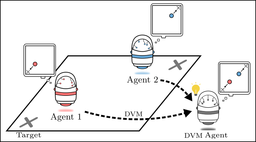
3. Multi-Agent Reinforcement Learning (MARL), which focuses on the interactions of multiple agents, and meta-learning, where agents learn to adapt their learning strategies. These advancements will enhance the adaptability and efficiency of RL algorithms, paving the way for applications across various fields, including robotics, healthcare, and personalized recommendations.

Present and Future Applications :

1. A great example is the use of AI agents by Deepmind to cool Google Data Centers. This led to a 40% reduction in energy spending. The centers are now fully controlled with the AI system without the need for human intervention.
2. IBM for example has a sophisticated reinforcement learning based platform that has the ability to make financial trades. It computes the reward function based on the loss or profit of every financial transaction.
3. In this paper, the authors propose real-time bidding with multi-agent reinforcement learning. The handling of a large number of advertisers is dealt with using a clustering method and assigning each cluster a strategic bidding agent. To balance the trade-off between the competition and cooperation among advertisers, a Distributed Coordinated Multi-Agent Bidding (DCMAB) is proposed. 
4. In marketing, the ability to accurately target an individual is very crucial. This is because the right targets obviously lead to a high return on investment. The study in this paper was based on Taobao — the largest e-commerce platform in China. The proposed method outperforms the state-of-the-art single-agent reinforcement learning approaches.